import os
from iqm.qiskit_iqm import IQMProvider

os.environ["IQM_TOKEN"] = "TODO: Add your VTT QX API token here"
provider = IQMProvider(
    url="https://qx.vtt.fi",
    quantum_computer="q50",  # Replace with 'q5' or 'demo' as needed
)
backend = provider.get_backend()Exploring the Device Quantum Architecture
This notebook introduces the two types of quantum architecture, that are exposed by each device on VTT QX:
- Static quantum architecture: Describes the qubits and couplers present on the QPU and their connectivity.
- Dynamic quantum architecture: Describes the qubits and couplers that are currently available through the software control stack.
The notebook explains how to query each object and how they differ. We start by initializing the Qiskit client that we’ll use for our exploration.
Initializing the Qiskit client
To initialize the Qiskit client, copy your VTT QX API token into the line marked with TODO.
Static Quantum Architecture
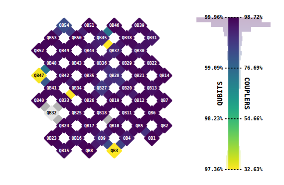
In the picture below, taken from the VTT QX dashboard, the VTT Q50 device topology is visualized. We see that QB32 and its surrounding couplers, as well as the coupler QB10-QB18 are displayed in gray, indicating that no calibration information is available. For VTT Q50, those qubits and couplers have been deactivated and are not usable.
We can fetch the same data used to generate the QPU visualization by manually querying the VTT QX API
import requests
from pprint import pprint

qx_url = "https://qx.vtt.fi/api/devices/q50"
url = f"{qx_url}/quantum-architecture"
headers = {
    "Accept": "application/json",
    "Authorization": f"Bearer {os.environ['IQM_TOKEN']}",
}
r = requests.get(url, headers=headers)
quantum_architecture = r.json()["quantum_architecture"]

# pprint(quantum_architecture)
We can check the number of qubits:
print(f"Number of qubits: {len(quantum_architecture['qubits'])}")Number of qubits: 54which matches the number of qubits shown in the figure. For running quantum algorithms, it is generally not useful to include deactivated qubits as they must be filtered out during the transpilation procedure. Therefore, another representation of the quantum architecture exists that excludes deactivated qubits, the dynamic quantum architecure.
Dynamic Quantum Architecture
The dynamic quantum architecture, is generated after every calibration run, which, in theory, allows us to dynamically exclude qubits with low fidelity (this feature is currently not in use). The dynamic quantum architecture, is the default data that is fetched by client libraries such as Qiskit or Cirq to initialize the coupling map and learn about supported operations.
For example, when we query the Qiskit backend, we see that it is aware of the missing qubit, as it shows 53 instead of 54 qubits
print(f"Number of qubits: {backend.num_qubits}")Number of qubits: 53Next, we print the mapping of index to qubit name:
for i in range(backend.num_qubits):
    print(f"{i} --> {backend.index_to_qubit_name(i)}")
We see that while indices are continuous, there is a jump in the qubit naming between QB31 and QB33 as QB32 has been excluded. This means that for all qubits with index below 31, the corresponding name is QB{index + 1} and for qubits with index greater or equal than 31, the corresponding name is QB{index + 2}.
Note: A particular DQA is always tied to a calibration set ID. Therefore, the index to physical qubit mapping shown above might not apply to the calibration you are usng. To avoid confusion, it is recommended to use the backend function qubit_name_to_index when defining a fixed mapping for your quantum circuit. An example is shown below:
from qiskit import QuantumCircuit

qubits = ["QB24", "QB25", "QB33"]

qc = QuantumCircuit(len(qubits))

qc.h(0)
qc.cx(0, 1)
qc.cx(1, 2)
qc.measure_active()

qc.draw("mpl", idle_wires=False)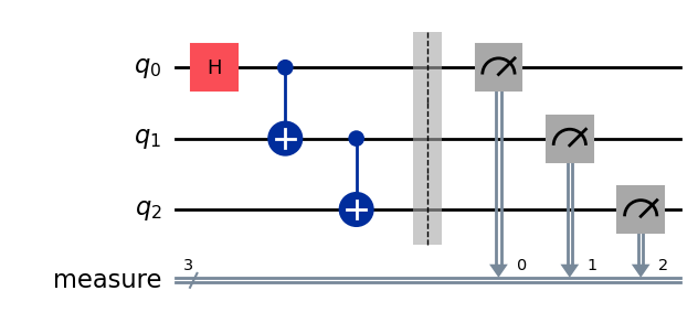
from qiskit import transpile

initial_layout = [backend.qubit_name_to_index(q) for q in qubits]
transpiled_circuit = transpile(
    qc, backend=backend, initial_layout=initial_layout, optimization_level=1
)

transpiled_circuit.draw("mpl", idle_wires=False)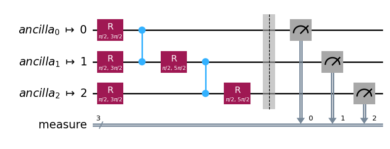
After executing the quantum circuit, we can verify that the mapping has actually been applied
results = backend.run(transpiled_circuit, shots=1024).result()
pprint(results.request.circuits[0].instructions)
(Instruction(name='prx', implementation=None, qubits=('QB24',), args={'angle_t': 0.25000000000000006, 'phase_t': 0.75}),
Instruction(name='prx', implementation=None, qubits=('QB25',), args={'angle_t': 0.25000000000000006, 'phase_t': 0.75}),
Instruction(name='cz', implementation=None, qubits=('QB25', 'QB24'), args={}),
Instruction(name='prx', implementation=None, qubits=('QB25',), args={'angle_t': 0.25000000000000006, 'phase_t': 1.25}),
Instruction(name='prx', implementation=None, qubits=('QB33',), args={'angle_t': 0.25000000000000006, 'phase_t': 0.75}),
Instruction(name='cz', implementation=None, qubits=('QB25', 'QB33'), args={}),
Instruction(name='prx', implementation=None, qubits=('QB33',), args={'angle_t': 0.25000000000000006, 'phase_t': 1.25}),
Instruction(name='barrier', implementation=None, qubits=('QB24', 'QB25', 'QB33'), args={}),
Instruction(name='measure', implementation=None, qubits=('QB24',), args={'key': 'measure_3_0_0'}),
Instruction(name='measure', implementation=None, qubits=('QB25',), args={'key': 'measure_3_0_1'}),
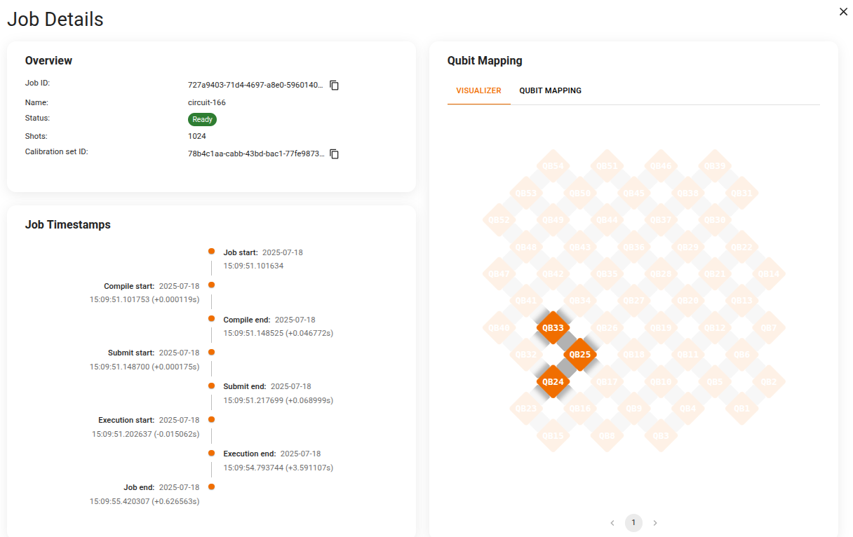
Instruction(name='measure', implementation=None, qubits=('QB33',), args={'key': 'measure_3_0_2'}))Alternatively, we can check the VTT QX job view to verify, that the mapping has been correctly applied